Pricing Options with TorchSDE
The basic operation of finance is to estimate distributions of forward values on assets, and buy/sell them accordingly. Usually buying/selling does not allow the purchaser to monetize all the information the investor might have about an asset. Options by contrast allow the investor to monetize all information he/she might have about the forward distribution of an asset. A simple derivation shows that the second derivative of call prices with respect to strike (K) are proportional to the forward density on the underlying (S) at expiry. Starting from the payoff of European call written with the Heaviside function \(\Theta\):
\(C = \langle \Theta(S(t)-K)*(S(t)-K) \rangle\) \(\rightarrow \frac{d^2 C}{dK} \propto \langle \delta(S(t)-K) \rangle\)
In any reasonable picture, the prices of any asset are strongly driven by noisy variables which cannot be observed. This makes stochastic differential equations the go-to tool to understand price trajectories of assets. Modern versions of these equations propagate stochastic volatilities alongside the underlying, for example the Heston model:
\[dS_{t}=\mu S_{t}\,dt+{\sqrt {\nu_{t}}}S_{t}\,dW_{t}^{S}\] \[d\nu_{t}=\kappa (\theta -\nu_{t})\,dt+\xi {\sqrt {\nu_{t}}}\,dW_{t}^{\nu }\]The dynamics of volatility(\(\nu(t)\)) determined by the stochastic parameters in this equation induce different prices for options at different strikes and expiries. This is called a “Volatility Surface”. Day to day on even the most liquid chains of options, these parameters hop up and down, as the market gyrates between beliefs about what these parameters will trade at tomorrow. Best-fit parameters of the moment, imply the market’s belief in the forward distribution of assets values, and allow one to draw trajectories of what the underlying might do, according to the market (within the model).
Usually the act of calibrating an SDE to market data requires a lot of domain specific technology. Differentiable programming is changing all that. Recently, a group at google released a library (torchSDE) which allows anyone to differentiably solve stochastic DE’s. In particular this means that functions of stochastic trajectories (fit to surface) can be optimized as a function of stochastic parameters. Let’s look at a simple Heston fit of the VIX call surface. The first step is to define a torch module which encodes the drift and diffusion of the process:
class Heston(torch.nn.Module):
    noise_type = 'general'
    sde_type = 'ito'
    """
    Simple implementation of Heston Model.
    To learn the vol along with the other parameters...
    Sigma0 needs to be a shifted parameter.
    Annoyingly.
    """

    def __init__(self, S0 = 100.,
                       sigma0 = .12,
                       mu = 0.07,
                       kappa = 2.60,
                       theta = 0.12,
                       xi = 0.5
                ):
        super().__init__()
        self.S0 = S0
        if (2*kappa*theta - xi*xi<0):
            print('VIOLATES FELLER, NONPOSITIVE')
        inv_softplus = lambda x: x + tch.log(-tch.expm1(-x))
        self.sigma0 = tch.nn.Parameter(torch.ones(1)*sigma0
                                   , requires_grad = True)
        self.skew_ = tch.nn.Parameter(tch.ones(1)*1e-4
                                   , requires_grad = True)
        self.mu = tch.nn.Parameter(torch.ones(1)*mu
                                   , requires_grad = True)
        self.kappa = tch.nn.Parameter(torch.ones(1)*kappa
                                   , requires_grad = True)
        self.theta = tch.nn.Parameter(torch.ones(1)*theta
                                   , requires_grad = True)
        self.xi = tch.nn.Parameter(torch.ones(1)*xi
                           , requires_grad = True)
        self.brownian_size = 2
        self.state_size = 2
    @property
    def v0(self):
        return self.sigma0*self.sigma0
    @property
    def rho(self):
        return tch.tanh(self.skew_)
    def __repr__(self):
        return f"sigma: {self.sigma0.detach().item():.3f} rho: {self.rho.detach().item():.3f} mu: {self.mu.detach().item():.3f} kappa: {self.kappa.detach().item():.3f} theta: {self.theta.detach().item():.3f}  xi: {self.xi.detach().item():.3f}"
    def y0(self, ntraj=100):
        return tch.tensor([self.S0, tch.zeros_like(self.S0)]).expand(ntraj,2)
    def f(self, t=None, y=None):
        batch_size = y.shape[0]
        state_size = y.shape[-1]
        dsdt = self.mu*y[:,0]
        nu=(y[:,1].abs()+self.sigma0*self.sigma0+1e-14)
        dvdt = self.kappa*(self.theta - nu)
        return tch.stack([dsdt, dvdt],-1)
    def g(self, t=None, y=None):
        """
        Returns
            g_tensor: batch X state X brownian
        """
        batch_size = y.shape[0]
        state_size = y.shape[-1]
        nu=(y[:,1].abs()+self.sigma0*self.sigma0+1e-14)
        dsdw = nu.sqrt()*y[:,0]
        dvdw1 = self.rho*self.xi*nu
        dvdw2 = tch.sqrt(1. - self.rho*self.rho)*self.xi*nu
        return tch.stack([dsdw, dvdw1, tch.zeros_like(dsdw), dvdw2],-1).reshape(-1,2,2)
Next we can define a simple routine which can take a dataframe representing the options chain (it has pretty obviously named columns) and optimize the fit of the market prices using this model by integrating the SDE, and minimizing the price errors. I’ve used some simple classes from my private codebase for manipulating named tensors, but the functionality would be trivial for anyone following along.
def expected_prices(dexps, strikes, times, spot_trajs,
                    sign, rate, divrate):
    """
    The expected call price is simply
     <Relu(S - K)>
    """
    Ti = (times.unsqueeze(0) < dexps.unsqueeze(-1)/365.).sum(-1)
    final_samples = spot_trajs[Ti,:]
    rate_discount = tch.exp(-1*rate*dexps/365.)
    spot_adjustment = tch.exp((rate-divrate)*dexps/365.)
    call_prices = rate_discount*((final_samples*spot_adjustment.unsqueeze(-1) - strikes.unsqueeze(-1)).relu_()).mean(-1)
    put_prices = rate_discount*((strikes.unsqueeze(-1)-final_samples*spot_adjustment.unsqueeze(-1)).relu_()).mean(-1)
    return tch.where(sign<0, put_prices, call_prices)

def optimize_sde_on_chain(chain_frame,
                          sde_: tch.nn.Module,
                          max_steps = 50,
                          ntraj = 15000,
                          only_calls = True
                         ):
    if (only_calls):
        chain_tensor = raw_to_named_tensor(chain_frame[chain_frame.sign>0])
    else:
        chain_tensor = raw_to_named_tensor(chain_frame)
    nt=int(chain_frame.dexp.max()*1.01)
    max_t = (chain_frame.dexp.max()+1)/365.
    ts = torch.linspace(0, max_t, nt)

    strikes = chain_tensor.get('strike')
    rate = chain_tensor.get('rate')
    divrate = chain_tensor.get('divrate')
    last_ulying = chain_tensor.get('last_underlying')
    dexps = chain_tensor.get('dexp')
    sign = chain_tensor.get('sign')
    prices = chain_tensor.get('qmid')

    sde_.S0 = last_ulying.mean()
    print("S0: ",sde_.S0.item())

    optimizer = tch.optim.Adam(sde_.parameters(),
                               lr=0.02,
                               weight_decay=0.0,
                               amsgrad=False)

    for iter in range(max_steps):
        optimizer.zero_grad()
        ys = torchsde.sdeint(sde_, sde_.y0(ntraj=ntraj), ts)
        if (iter%10==0):
            _=plt.plot(ys[:,:,0].detach(),alpha=0.02)
            _2=plt.plot(ys[:,:,0].detach().mean(-1), alpha=0.5, c='r', label='Mean')
            plt.title('Spot')
            plt.ylim(0,100)
            plt.show()
        eps = expected_prices(dexps, strikes, ts, ys[:,:,0], sign, rate, divrate)
        loss = tch.pow(prices - eps, 2.0)
        loss_value = loss.mean()
        print(iter," RmsPrice ", loss_value.detach().sqrt().item())
        print(sde_)
        loss_value.backward(create_graph=True)
        optimizer.step()
    # plot the surfaces?
    return
The convergence process of the fit looks like this:
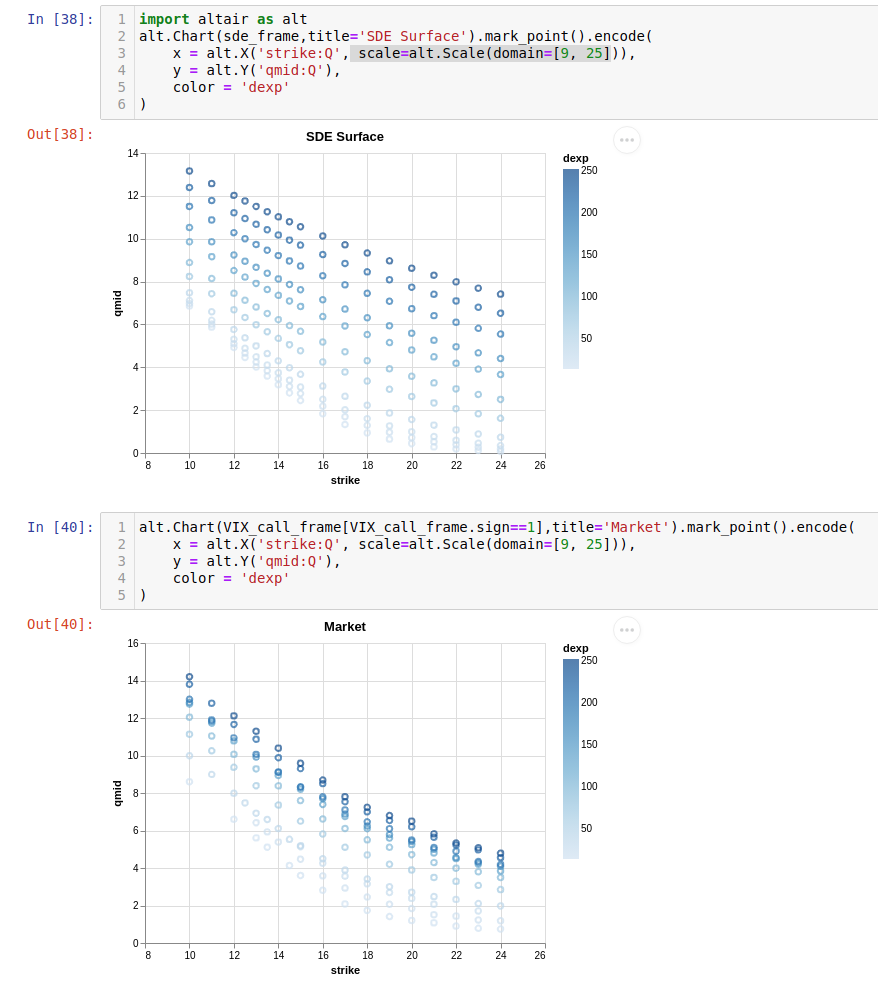
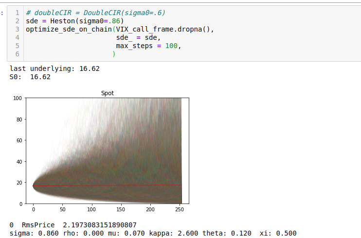 Heston is a rather terrible model for VIX futures, and so even at convergence there’s an rms error of 1.5$ dollars per option. However the essential shape of the VIX surface is somewhat cartoonishly fit.
Importantly with this converged SDE, Greeks of any order and hedges of any type can be made. One could hedge derivative positions arbitrarily well even operating with home-gamer levels of resources. Of course a nicer thing to do would be to use a fractional brownian vol process, but that’s not currently supported by torchSDE. Perhaps two papers down the line it will be though.