How to Size Bets. The Kelly Criterion in PyTorch
Suppose you would like to make a wager on a random outcome because you believe you know something about the probability of the outcome, for example that 265/365 days in a year will be cloudy in South Bend, Indiana. How much should you wager it will be cloudy tomorrow if you would be paid even odds, under the assumption you will take bets for an eternity and instantly.
If your statistics are good there’s a unique correct answer due to John L. Kelly Jr., American treasure. You should wager ~45% of the money you have because it maximizes the exponential rate of growth (G) of your wealth (W) in the limit of a large number of bets (N). You find the desired sizing (c, a fraction of your capital) by maximizing what you can easily work out is G after many trials: G=(win fraction) log(1+c)+(lose fraction)log(1-c). There’s a unique c that maximizes this G expression as a function of c. You can find c using the optimization method of your choice. This number balances the value of the information you have, with the payoff of the bet. Gamblers are very familiar with this elementary version of the “Kelly Criterion”. What is documented in fewer places is how to use this in a general setting, where the payoff distribution is complex, multi-dimensional, or only available as samples. That’s what I’ll describe here.
NOTE: The interesting thing about Kelly’s paper: “A novel interpretation of the information rate” is that the rate of growth of your wealth, is actually the same as the information rate (in the Shannon - Information theory sense) of the channel which you are getting your probability information from. Kelly cared more about G, because it exposes a truth about information. It’s a classic relationship showing that entropic information has real-life units. This was certainly a deep and interesting insight. To anyone who has spent a life shoving facts in their brains it’s certainly comforting.

Kelly grew up not far from where I’m living in Austin. He attended UT down the road, before ending up at Bell Labs. Besides working with Shannon on the information rate stuff, Kelly was involved in some of the earliest text to speech systems in the years before his death. That work actually lead to the voice of HAL singing ‘Daisy’ at the end of ‘2001’. Even today this work continues today albeit with much more powerful neural-network compression. He died suddenly at the age of 41, as good people often do. It’s pleasant to think of him down the road watching the Austin sunset and firing a gun - randomly into the air like a true Texan. From our offices you can see the spot where Kelly cut his teeth.
Kelly + Monte Carlo & Correlated Bets
What about a much more sophisticated version of Kelly’s problems? Suppose you would like to place a complex wager on a 1000-dimensional random outcome. This could (for example) be the price of 1000 cryptocurrencies tomorrow, or 1000 businesses if you’re a VC, and you will wager on each of them separately out of your same pot of limited wealth. However suppose that instead of independent probability distributions for these 1000 outcomes (that wouldn’t be realistic) you have 1*10⁶ samples (S=1,000,000) of the 1000 variable outcomes (a matrix of dimension 1000 X a million). A sample is merely an example of what could happen. For example it could just be the historical list of daily returns for the 1000 cryptocurrencies, or you could draw samples from some simulation.
Samples are better than simple probabilities per asset because all the realistic correlations these events might have are captured. We’ll assume we have some large soup of these samples all equally likely, as one does in Monte Carlo. I’ll show you how to make samples in the next section. How do you use Kelly’s ideas (which are usually formulated in terms of probabilities) with these discrete samples? Following the math in Kelly’s paper with minor substitutions the answer is:
\[min_{c_k} \frac{-1}{S} \sum_i \text{log}\{\sum_k (1+c_kr_{ik})\}\]where \(r_{ik}\) is the return on the i-th sample for the k-th asset. (It’s the number you multiply by your wealth to determine the wealth-change after the outcome of a bet, i.e. r = +1 for a winning even-odds coin flip). \(c_k\) is the desired fraction of your wealth to wager on asset k. The main purpose of this article was for me to write down this formula, since I hadn’t seen it elsewhere.
To choose the correct \(c_k\) we need to perform a minimization, which involves differentiation. Back in Kelly’s days this would have taken a week of math and laborious coding, but thanks to packages like PyTorch, we can do this in a few seconds.
Kelly’s minimization doesn’t know silly things like you can’t bet with negative money. In order to enforce the “no infinite credit” constraint in a minimization we need to use Lagrange’s method of undetermined multipliers. Something that I am continuously horrified people often don’t know. That’s a separate lesson though, and I’m happily done teaching college. Suffice it to say you add a variable and a term to the loss, and then you can enforce \(\sum(c_k) <= 1.\)
Should we take this out for a spin? I would like to give you return samples for some financial assets… but that’s how I make my monies, so we need some toy problem to see the power of this technique. Since not everyone has a pretty lady to fly them to Vegas, I thought a fun one to try at home would be non-transitive dice. This will show you easily how to generate samples and use the math. Applying the Kelly Sizing optimizer will also show us some facts about betting in general.
Application to Non-Transitive Dice Game
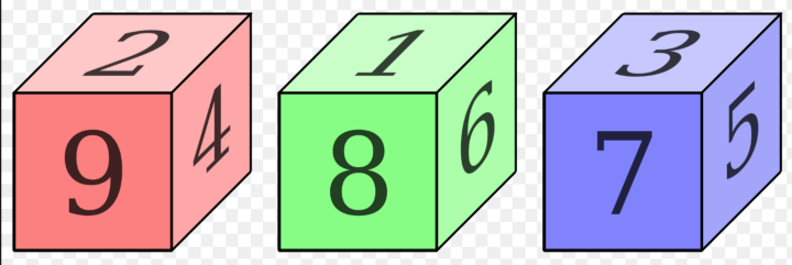
Suppose you got three dice with the following six face values:

dice1 = [2, 2, 4, 4, 9, 9.]# Play with some non-transitive dice.
dice1 = [2, 2, 4, 4, 9, 9.]
dice2 = [1, 1, 6, 6, 8, 8.]
dice3 = [3, 3, 5, 5, 7, 7.]
dice = [dice1, dice2, dice3]dice1 = [2, 2, 4, 4, 9, 9.]
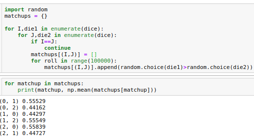
These dice obey a non-transitive rock-paper-scissors hierarchy of wins in the limit of a large number of match-ups. Die 1 beats 2, 55% of the time, etc. This code shows you how to do some math on the matchups (import numpy as np).

Interesting right? But all these dice have the same mean value (which is 5). Suppose that each of these dies will pay off it’s face value, divided by ten, minus .49 in a game we can play. That’s going to be a good bet, because the average payoff will be positive (1%, since the mean is (5/10)-.49). I would take that bet but I wouldn’t bet the farm.
- How much do you wager on each die alone? Would it be the same?
- How much together? Are those the same?
- The third die loses to the second, so it should have a smaller Kelly sizing, right?
- Do you bet less if you roll a die with the one it loses to?
Let’s channel Kelly y’all, smoke ‘em if you got em, and put your feet up. Basically all we’ll do is generate return samples and toss them in the routine above to get our answers.
Results
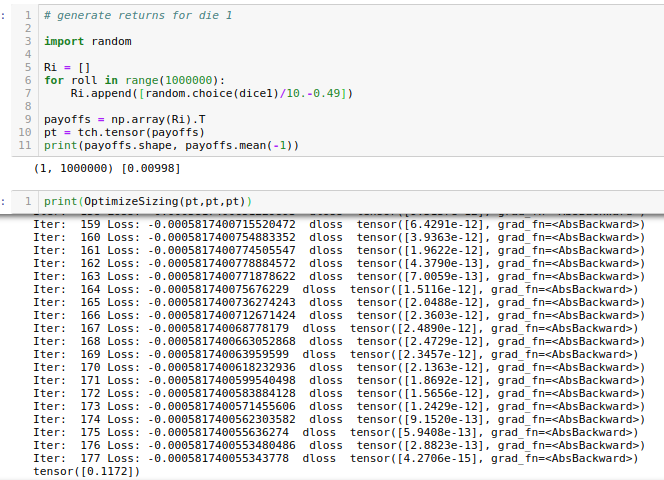
All we need to do is generate input tensors for the Kelly sizing optimizer by running trials to create return samples. Here’s that bit for die 1:

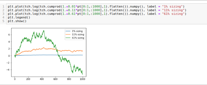
I have taken no care whatsoever to converge the Monte Carlo, I leave that pedantic crap to the reader. You can see the 1% mean payoff and ideal sizing of ~11% for the bet. Let’s look at some wealth trajectories if you bet much more or much less than that. I will do so on a log-scale to make everything visible.

Only the Kelly sizing does really well even after only 1000 bets. The 6x overbet blows out, and these were merely one set of possible realizations of these trajectories. Seems like the magic Texan has given us sound advice so far. What are the Kelly bets for rolling the three dies individually? Remember they all have the same average payoff per roll….Optimal 1-die Kellys: (dice1 11.7%, dice2 11.5%, dice3 36.5%)
This first surprising result shouldn’t be so surprising to people with a little investment/gambling experience. You shouldn’t wager the same amount on these dice. Although the mean payoff is the same for all, the standard deviation of the payoff is not. If you lose a lot you will have less to bet and so you will make less in the long run betting on things with the possibility of catastrophic loss even if the mean yield is the same. The last die has the smallest max drawdown by a factor ~2, and unsurprisingly that makes it a 2x better investment! Hedge fund people use a number, the Sharpe ratio (mean return over standard deviation of return) to describe this effect. Indeed the Sharpe ratio predicts the order of the optimal Kelly sizing if you are looking at these dies alone.
The usefulness of this Kelly Monte-Carlo optimizer is obvious. It makes you money from information. In this case, information in the form of samples. Note the Kelly sizer even works if your samples have some correlation, although dice clearly do not.
(Dedicated to X.)