Simply Extracting information out of your Stochastic Series
The unreasonable usefulness of Stochastic DE’s
Certain regions of science are unfortunately mired in formalism, despite the fact that they are invaluable. Stochastic calculus is without a doubt, one of these fields. A typical text on stochastic calculus will cover a series of formal theorems proving the existence of these integrals, but leave the reader without a clear picture of just how insanely practical these equations can be. If you’re modeling any type of noisy timeseries, it would be a huge mistake to not spend at least some time considering a stochastic DE as your zeroth order model. This post will cover the elementary math you need to fit a stochastic equation onto observed data by MLE, and how useful these equation are for extrapolation, normalization, featurization etc. As far as 1-d data goes, pretty much all of it is applicable to real world noisy incomplete data.
Brownian example
Suppose you have observed the coordinates of a particle drifting to the right, but also subject to random forces. You have a data series \(\{t, X_t\}\). You would like to answer elementary questions such as: “What’s an appropriate drift parameter with good time units based on these samples?” “How much is the particle affected by noise?” “How can I extrapolate trajectories of the particle in the future?”
One path to answering those questions is to model the particle as a Brownian Diffusion by first assuming a stochastic differential equation model of the form:
\[dX_t = \mu dt + \sigma dW_t\]This statement is a little loaded, especially the \(dW_t\) bit. But those unconcerned with formalism could focus on the finite difference approximation of \(X_t\). In this case \(dW_t\) is just a normal distribution of variance dt:
\[X_{t+1} \approx X_t + dt*\mu + N(0,dt)*\sigma\]Rearranging this to get the normal distribution on one side this expression implies a negative-log-likelihood objective to fix the parameters of the model:
\((X_{t+1}-X_t-dt*\mu)/\sigma \sim N(0,dt)\) … Which implies that the values on the left can be maximum-likelihood estimated. using the usual formula for the normal density: \(f(x)= {\frac{1}{\sigma\sqrt{2\pi}}}e^{- {\frac {1}{2}} (\frac {x-\mu}{\sigma})^2}\) The code below implements integration of the stochastic equation and maximum likelihood estimation of these parameters.
def stochastic_rk(X0, a, b, t, ntraj=8000, dW_ = None):
"""
Integrate stochastic runge-kutta
solves: dXt = a(Xt) dt + b(Xt)dWt
Args:
X0 : start of integration
a(X): dt component
b(X): dW component
t: array of timesteps
dW: if desired, a user-defined W process to do correlated assets.
"""
Ys = [X0]
n = t.shape[0]
if (dW_ is None):
dt = np.tile(np.abs(t[1:]-t[:-1])[:,np.newaxis],(1,ntraj))
dW = np.random.normal(np.zeros_like(dt),
np.sqrt(dt))
else:
dW = dW_*np.concatenate([np.zeros(1), np.sqrt(np.abs(t[1:]-t[:-1]))],0)
for i in range(1,n):
Yn = Ys[-1]
dt = t[i] - t[i-1]
sqrth = np.sqrt(np.abs(dt))
YYn = Yn + a(Yn)*dt + b(Yn)*sqrth
Ynp1 = Yn + a(Yn)*dt + b(Yn)*dW[i-1] + 0.5*(b(YYn)- b(Yn))*(dW[i-1]*dW[i-1]-dt)*sqrth
Ys.append(Ynp1)
return np.stack(Ys,0)
def nll_brownian(values, params, times=None, condition = 'tm1'):
"""
Because of the markov property the likelihood of each sample is independent.
so the log-likelihood is the sum.
"""
mu = params['mu']
sigma = params['sigma']
t = times - params['t0']
S0 = params['S0']
sigma2 = sigma*sigma
if (condition == 'tm1'):
dt = t[1:] - t[:-1]
log_prefactor = (-1./2.)*tch.log(2.*np.pi*sigma2*dt)
to_exp = tch.pow(values[1:] - values[:-1] - mu*dt,2.0)*(-1./(2*sigma2*dt))
nlls = -log_prefactor-to_exp
return tch.cat([tch.zeros_like(nlls[:1]), nlls],0)
elif condition == 'S0':
log_prefactor = (-1./2.)*tch.log(2.*np.pi*sigma2*t)
to_exp = (-1./(2*sigma2*t))*tch.pow(values - S0 - mu*t,2.0)
nlls = -log_prefactor-to_exp
return nlls
def fit_brownian(values_, times_=None, mode=None):
tore = {'model':'brownian'}
msk = ~tch.logical_or(tch.isnan(values_), tch.isinf(values_))
if msk.sum() < 2:
raise Exception('Insufficient Series Data')
times = times_[msk]
values = values_[msk]
if mode is None:
start_test = int(times.shape[0]*.9)
train_times = times[:start_test]
train_values = values[:start_test]
test_times = times[start_test:]
test_values = values[start_test:]
train_ps = fit_brownian(train_values, train_times, mode='train')
if (train_ps['mean_nll'] == np.inf):
tore['mean_nll'] = np.inf
tore['test_nll'] = np.inf
return tore
test_nlls = nll_brownian(test_values, train_ps, test_times)
tore['test_nll'] = test_nlls.mean()
t0 = times.min()
t1 = times.max()
dt = t1 - t0
tore['t0'] = t0
tore['t1'] = t1
tore['S0'] = values[0]
dX = values[1:] - values[:-1]
dT = times[1:] - times[:-1]
sigma_guess = ((dX - dX.mean())/tch.sqrt(dT)).std()
mu = tch.nn.Parameter(tch.tensor((dX/np.sqrt(dT)).mean()), requires_grad=True)
sigma_pre_softplus = tch.nn.Parameter(tch.tensor(softplus_inverse(sigma_guess)), requires_grad=True)
tore['mu'] = mu
tore['sigma'] = tch.nn.functional.softplus(sigma_pre_softplus)
model_params = [mu, sigma_pre_softplus]
optimizer = tch.optim.Adam(model_params, lr=0.001)
last_loss = 5000.
for I in range(8000):
tore['mu'] = mu
tore['sigma'] = tch.nn.functional.softplus(sigma_pre_softplus)
loss = nll_brownian(values[20:], tore, times[20:]).mean()
loss.backward()
if np.abs(last_loss - loss.item()) < 1e-4:
break
else:
last_loss = loss.item()
tch.nn.utils.clip_grad_norm_(model_params,10.)
optimizer.step()
optimizer.zero_grad()
tore['sigma'] = tore['sigma'].detach().cpu()
tore['mu'] = tore['mu'].detach().cpu()
nlls = nll_brownian(values, tore, times)
if (tch.any(tch.isnan(nlls))):
tore['mean_nll'] = np.inf
else:
tore['mean_nll'] = nlls.mean()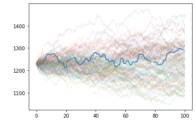
tore['std_nll'] = nlls.std()
return toreHere’s an example of what this looks like if you appropriately MLE SPX and then draw a large number of trajectories.

Information Is Noise
Once you’ve optimized parameters of a stochastic equation, you can propagate it forwards and backwards in time, which is useful. You can draw trajectories from it, but perhaps the most useful thing you can do is replace X with it’s noise process, by simply solving for dW which resulted in a particular trajectory. This results in a series with the same information as X, but which is quasi-normally distributed. This reduces all the information in the series in a form most-amenable to statistics.
\[\text{SPX}_t \rightarrow dW_t \rightarrow \text{IWM}_t\]To make one powerful final example. IWM (a Russell ETF) has a strong correllation to SPX. In the following plot I have MLE fit a particular (non-brownian) 4-parameter stochastic equation on both SPX and IWM. Then I obtain SPX’s dW noise process and then integrate it using the parameters of IWM:
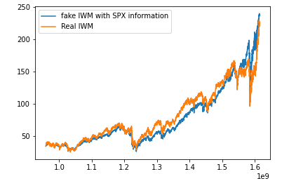
The crazy thing about this plot is that the fake blue series only has four pieces of information about IWM. Besides that all it’s using is the fact that SPX and IWM’s noise processes are the same. How many noise processes of different assets you hold are the same?