Using simple mean-reversion to remove carry from a VIX futures position

Time for a practical finance lesson for beginners.

What are VIX futures.

If you know what a VIX future is, skip ahead. VIX is theoretical index, a single instantaneous number, designed to capture the market implied volatility on the dominant American stock index. The most elementary model of a stock or stock basket’s price is geometric brownian motion, \(dX_t = \mu X_t dt + \sigma X_t dW_t\). Assuming this model, the prices of European options are set by a simple analytically tractable solution to this SDE leading to the unjustly famous Black-Scholes formula. Of course the market does not believe this formula applies at all times. Usually the market likes to imagine the asset prices obeying this formula at zeroth order, with changes corresponding to a time-dependent diffusion (or volatility) parameter \(\sigma(t)\). By inversion Black-Scholes implies a volatility for each option price. Roughly speaking VIX \(= \sigma(t)\) implied by the market on S&P options at a given time. When the market anticipates great change coming, VIX shoots up (often by several multiples). Volatility is mean reverting. It makes no sense for stock to be either infinitely volatile, or static, and so volatility is constrained between bounds, generally between 10-ish percent and 100 percent for VIX.

The market for the VIX futures was born a few years before the ‘08 crisis. More than a decade later, it’s still a liquid market. These let you take a position that volatility might increase or decrease a time in the future. If you are long a one-month VIX future, you would get cash settled for a version of the VIX spot price when your future expires, hopefully above what you paid for the future if you’d like to profit. Because they go up by multiples of their cost when the market tanks, VIX futures are an excellent hedge for index risk exposure. For all intents and purposes, buying VIX futures is paying the price of risk, in the hopes risk will go up.

When the market for VIX futures opened, to be honest people knew a lot less about \(\sigma(t)\) than they know today, and the futures were simply mis-priced. For several years there was all sorts of durable arb between S&P positions and VIX futures and options. Since then people like Lorenzo Bergomi and Jim Gatheral have advanced really sophisticated, non-Markovian models for volatility which satisfy small nuances of empirical behavior of vol. The market largely prices these in now. This post concerns itself with a simple elementary understanding of the futures.

Institutional products behave in a rational way.

The way markets think, once a cost is known, it’s not really a risk so much as a discount. Thus it’s usually the case that risk in the distant future is priced above risk in the present. This causes the prices of VIX futures to be usually decreasing, on average by 0.0014% a day. If you were to buy a VIX future as an investment, and hold it, you would usually lose large amounts of money:

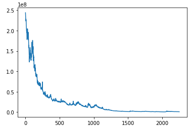
The above plot is the cumulative value of a strategy which maintains a 100,000$ position in a 21 day VIX future at all times. To lose 10**8 dollars in 2000 days is not attractive. How is it there is a liquid market on VIX futures? Well these are an institutional product, and institutional investors have models which allow them to avoid paying this cost. They would not simply buy and hold a VIX future, they would keep their position somehow hedged, so-as to overall benefit from being long this future. Can the simple people at home do the same? Yes.

A simple OU process let’s you hold a VIX future.

In a previous post, I show how one can easily use Pytorch and Maximum Likelihood Estimation to fix the parameters of simple 1D stochastic models. Because VIX is mean-reverting, a good zeroth-order choice would be an Ornstein-Uhlenbeck process:

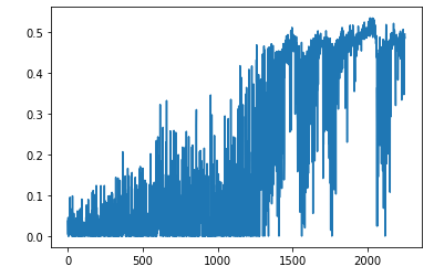
\[dX_t = \alpha(\mu - X_t) dt + \sigma X_t dW_t\]

If one simply MLE fits the loser-VIX future position to an OU process fixing the parameters (\(\alpha, \mu, \sigma\)), one obtains a model from which you can draw trajectories of the VIX futures, conditioned on global parameters, and most importantly the current price of the future, which captures the mean-reversion effect. Drawing a large number of trajectories from this process, one could either then size a VIX futures position using Kelly (see my how to bet post for an example), or one could use the simple rule-of-thumb that Kelly is usually roughly the maximum of sortino divided by two and zero. This yields the (pure-long) VIX exposure with the PnL below:

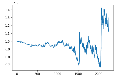
Perhaps unsurprisingly, this yields a synthetic, pure long position in a VIX future, which doesn’t bleed money, but rather roughly appreciates at the risk-free-rate. This asset can be combined with any portfolio of long equity to reduce risk in times of crisis, although it still does a worse job than an entire hedge fund devoted to holding a long vol position, such as my present employer. In case you’re curious, this would be the amount of 21-day VIX future you would hold as a function of days since 1999 simply accounting for the mean reversion information: